Microseismic Monitoring

Conceptual workflow for event detection and interpretation in potash mining.

Why Microseismic Monitoring Matters

Microseismic monitoring helps detect small-scale rock mass movements that are not visible through traditional inspection. In high-conductivity environments like potash mines, microseismic data supports ground control, safety, and operational decision-making.

Conceptual Workflow

Sensor Layout: Geophones or accelerometers installed in drifts or boreholes.
Noise Filtering: Removing machinery noise, ventilation noise, and background vibrations.
Event Detection: Identifying small seismic events within noisy data.
Event Location: Triangulating source position using arrival times.
Interpretation: Understanding rock mass behavior and potential instability.

Interactive Example – Raw vs Filtered Signal

This simple synthetic example illustrates how filtering improves event visibility.

Python Demo – Synthetic Microseismic Events

This short Python demonstration shows how synthetic microseismic events can be generated, filtered, and detected. It illustrates the first step of a real microseismic workflow: identifying event candidates within noisy data.

Level 1: Single-Trace Event Detection

The video below walks through the raw signal, the filtered signal, and the detection of local maxima (event candidates). This conceptual example is designed for educational purposes and mirrors the early stages of microseismic processing.

Level 2: Multi‑Geophone Synthetic Microseismic Example

Educational synthetic example using six geophones. A single microseismic event is recorded across the array, with arrival times adjusted for visualization. The left panel shows the filtered traces with detected peaks, and the right panel displays the corresponding travel‑time trend across the geophones.

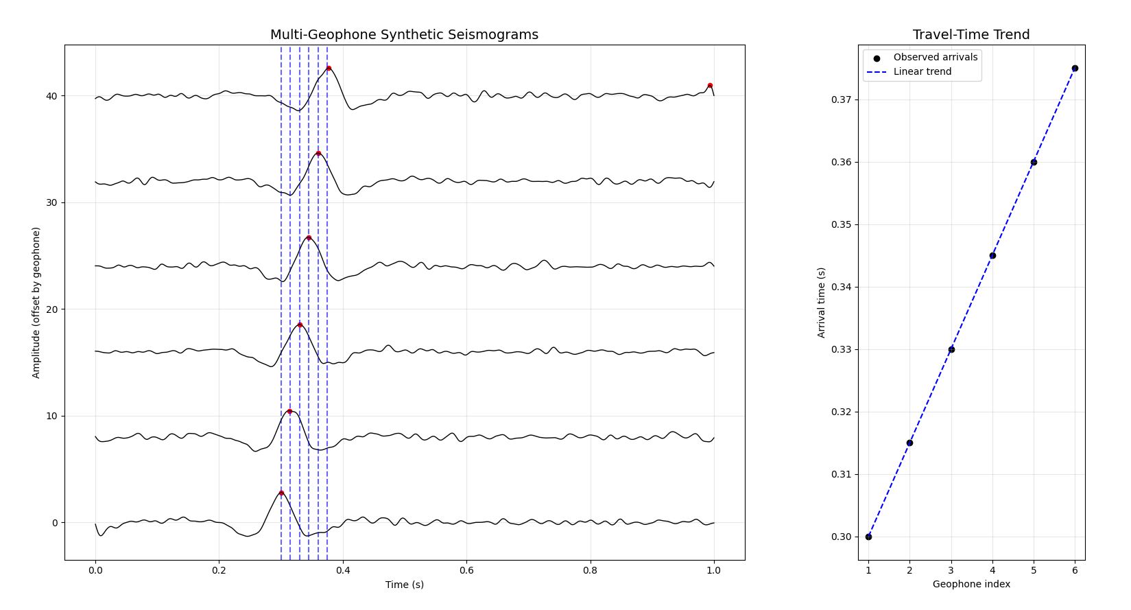
Level 2 – Multi-Geophone Synthetic Microseismic Event

Figure: A single synthetic microseismic event recorded across six geophones. Left: filtered traces with detected arrivals. Right: travel‑time trend used for basic quality control and interpretation.

Level 3: From Arrival Times to Event Location

Building on the multi‑geophone example from Level 2, this section demonstrates how arrival‑time differences can be used to estimate the location of a microseismic event. The goal is to illustrate the core idea behind travel‑time inversion using a simple synthetic example with six geophones.

3.1 Synthetic Setup

To remain consistent with Level 2, this example uses six geophones placed along a horizontal drift. A synthetic microseismic event is defined below the array, and theoretical travel times are computed using a constant velocity. Small perturbations are added to mimic realistic picking uncertainty.


    // Six geophones along a drift (meters)
    G = [
      {x: 0,  y: 0, z: 0},
      {x: 5,  y: 0, z: 0},
      {x: 10, y: 0, z: 0},
      {x: 15, y: 0, z: 0},
      {x: 20, y: 0, z: 0},
      {x: 25, y: 0, z: 0}
    ];

    // True event location
    E_true = {x: 12, y: 0, z: -18};

    // Velocity (m/s)
    v = 2500;

    // Travel-time function
    function travelTime(G, E, v) {
      let dx = G.x - E.x;
      let dy = G.y - E.y;
      let dz = G.z - E.z;
      let d  = Math.sqrt(dx*dx + dy*dy + dz*dz);
      return d / v;
    }

3.2 Arrival‑Time Inversion

Because the event origin time is unknown, the inversion uses arrival‑time differences between geophones. With six sensors, the system is over‑determined, which stabilizes the solution and reduces sensitivity to noise. A simple 2D grid‑search inversion is used for clarity.


    // Synthetic observed arrival times (with small noise)
    t_obs = G.map(g => travelTime(g, E_true, v) + (Math.random()*0.002 - 0.001));

    // Grid-search inversion
    function invertLocation(G, t_obs, v) {
      let best = {x: 0, z: 0, misfit: 1e9};

      for (let x = 0; x <= 25; x += 0.2) {
        for (let z = -40; z <= -5; z += 0.2) {
          let E = {x: x, y: 0, z: z};
          let t_calc = G.map(g => travelTime(g, E, v));

          let mis = 0;
          for (let i = 0; i < G.length - 1; i++) {
            let dt_obs  = t_obs[i+1] - t_obs[i];
            let dt_calc = t_calc[i+1] - t_calc[i];
            mis += Math.pow(dt_calc - dt_obs, 2);
          }

          if (mis < best.misfit) best = {x: x, z: z, misfit: mis};
        }
      }
      return best;
    }

    E_est = invertLocation(G, t_obs, v);

3.3 Estimated Event Location

The cross‑section below shows the six geophones, the true synthetic event, and the estimated event obtained from the arrival‑time inversion. The small offset between true and estimated location reflects realistic uncertainty due to noise, simplified velocity assumptions, and grid resolution.

Velocity (m/s): 2500

| | | | | | |

1500 2000 2500 3000 3500 4000 4500

Adjust the assumed P‑wave velocity used in the inversion. Higher velocity = faster travel times.

⚠️ Note: In real microseismic monitoring, the true event location is never known. Only the estimated location is available, and its accuracy depends heavily on the velocity model. Adjusting the velocity slider above shows how incorrect velocities distort the estimated position — which is why mines rely on sonic logs, calibration blasts, and iterative velocity updates.

⚙️ Future improvement: I plan to expand this section with more interactive controls to explore how velocity, geometry, and noise influence microseismic inversion.

Potash Stratigraphy and Seismic Velocities

Sylvite
2500–3000 m/s

Halite
~4500 m/s

Anhydrite
~6000 m/s

Carbonate
5500–6500 m/s

Stratigraphic order (top to bottom) and typical P-wave velocities. Solubility increases upward.

In Saskatchewan potash mines, the stratigraphy typically transitions from carbonate (limestone/dolomite) and anhydrite (CaSO₄) at the bottom to halite (NaCl) and sylvite (KCl) near the top. These evaporite units have distinct seismic velocities, and the strong contrast between them plays a major role in microseismic travel‑time behavior and inversion accuracy.

Material	Velocity (m/s)	Notes
Air	~330	Extremely compressible
Unsaturated weathering layer	300–1500	Loose grains, air-filled pores
Seawater	~1500	High bulk modulus, uniform
Soft marine sediments	1400–1800	Slightly lower or higher than seawater
Sylvite (KCl)	2500–3000	Main potash mineral
Potash ore mixture	2000–3000	Sylvite + halite + insolubles
Halite (NaCl)	~4500	Strong evaporite
Sandstone	2500–4500	Depends on compaction
Shale	2500–3500	Highly variable
Limestone	5500–6000	High stiffness
Dolomite	6000–6500	Very stiff
Anhydrite	~6000	Strong evaporite
Basement rocks	5500–7000+	High density, high modulus

Typical seismic velocities for common geological materials. Adapted from typical potash and evaporite velocity ranges reported in mining geophysics literature.

Improving Microseismic Location Accuracy

Microseismic accuracy depends strongly on the velocity model and the physical properties of the surrounding units. In practice, location quality can be improved by integrating additional geophysical methods such as:

GPR (Ground Penetrating Radar) – high‑resolution imaging of shallow structures.
EM / MT – mapping resistivity contrasts that correlate with lithology changes.
Seismic refraction – constraining near‑surface velocity variations.
Borehole geophysics – direct measurement of P‑ and S‑wave velocities.

These methods provide independent constraints that reduce uncertainty in the velocity model and improve the reliability of microseismic event locations.