Frequency‑Domain Electromagnetics
Electromagnetic fields in the frequency domain behave diffusively rather than as propagating waves. The penetration depth is controlled primarily by frequency, conductivity, and magnetic permeability, making frequency a direct lever on the depth of investigation (DOI). Lower frequencies penetrate deeper but provide lower resolution, while higher frequencies resolve shallow structure with greater detail. Understanding this relationship is essential for evaluating survey design, instrument performance, and claims about achievable DOI. In particular, frequency‑dependent attenuation explains why small transmitter–receiver spacing cannot produce deep penetration, and why sensor height has a measurable impact on detectability. This module explores these relationships through analytical expressions, interactive visualizations, and numerical simulations.
Abstract
This module explores the depth of investigation (DOI) in frequency‑domain electromagnetic (EM) methods. In contrast to time‑domain systems, frequency‑domain EM uses sinusoidal sources, and the penetration depth is controlled primarily by frequency, conductivity, and magnetic permeability. Lower frequencies penetrate deeper but provide coarser resolution, while higher frequencies resolve shallow structure with greater detail.
We introduce the key analytical relationships between frequency, skin depth, and attenuation, and examine how survey geometry and sensor height influence the effective DOI. A simple numerical model is then used to visualize frequency‑dependent attenuation and to clarify why small transmitter–receiver spacing and elevated sensor heights limit sensitivity to deeper targets, despite common claims of “deep penetration” in commercial systems.
Background Theory: Skin Depth, Frequency, and DOI
Skin Depth
Electromagnetic fields in conductive ground decay exponentially with depth. The characteristic decay length is the skin depth:
\( \delta = \sqrt{\frac{2}{\omega \mu \sigma}} \)
Skin depth controls how deeply a signal can penetrate:
- Large δ → slow attenuation → deep penetration
- Small δ → fast attenuation → shallow penetration
Frequency Relationship
Frequency directly controls skin depth:
- High frequency → large ω → small δ → fast attenuation → shallow DOI
- Low frequency → small ω → large δ → slow attenuation → deep DOI
In practical terms:
- 10 Hz penetrates deepest
- 1000 Hz penetrates shallowest
What δ Means for Survey Design
Different applications require different skin depths:
-
Small δ (high frequency)
- shallow DOI
- high resolution
- sensitive to near‑surface features
- used for UXO, archaeology, environmental mapping
-
Large δ (low frequency)
- deep DOI
- lower resolution
- used for groundwater, mineral exploration, deep structure
Interpreting the Attenuation Curves
- The 10 Hz curve decays slowly → deep penetration
- The 1000 Hz curve decays rapidly → shallow penetration
- The legend shows δ for each frequency, confirming the relationship
These curves provide a clear visual demonstration of how frequency controls depth of investigation (DOI), and why geometric tricks (like small Tx–Rx spacing) cannot overcome physical attenuation limits.
Depth of Investigation (Conceptual)
These static illustrations show how electromagnetic attenuation varies with depth and how sensor height influences the observed amplitude decay. Together, they provide a conceptual view of the depth of investigation (DOI) for different acquisition geometries.
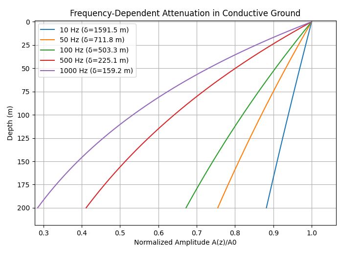
Normalized amplitude attenuation with depth for a representative frequency.
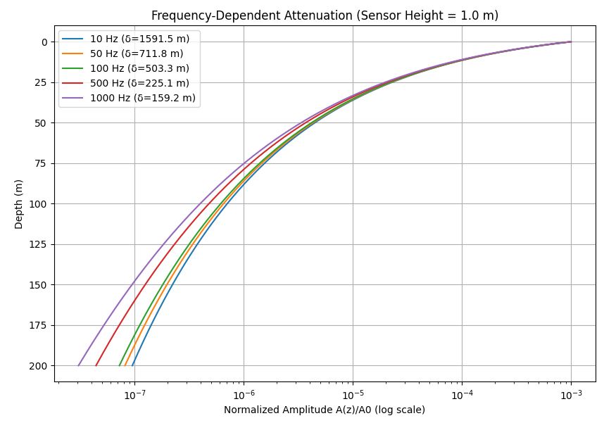
Effect of sensor height on the measured attenuation profile.
❓ What is \(A_0\)? Where is it measured?
\(A_0\) is the reference amplitude measured at the sensor height. This means:
- If the sensor is at 1 m, then \(A_0\) is the amplitude at 1 m.
- If the sensor is at 0 m (ground level), then \(A_0\) is the amplitude at 0 m.
❓ Why do the curves shift left or right on a log scale?
The plotted quantity is the normalized amplitude: \[ A_{\text{norm}}(z) = \frac{A(z)}{A_0} \] If the sensor height increases, \(A_0\) becomes larger. As a result, the ratio \(A(z)/A_0\) becomes smaller, and the curve shifts left on a logarithmic x‑axis. This left‑shift does not mean the signal is weaker — it only reflects the larger reference amplitude.
❓ Does a higher sensor height increase or decrease attenuation?
In absolute terms, attenuation decreases — the signal is stronger because the sensor is closer to the less‑attenuated region of the field. In normalized terms, the curve may appear more attenuated (shifted left) because \(A_0\) is larger. Both statements are correct because they refer to different reference points.
❓ Does a higher sensor height improve DOI?
Yes. A higher sensor height results in:
- Higher absolute amplitude
- Lower absolute attenuation
- Better signal‑to‑noise ratio (SNR)
❓ Does raising the sensor always improve DOI?
No — the improvement only holds up to a point.
Raising the sensor too high causes the field to weaken due to geometric spreading and air‑path attenuation.
Beyond a certain height, the ground contribution becomes too small and DOI decreases.
A useful analogy is a flashlight:
- Too close to the ground → tiny illuminated area.
- Raised slightly → larger, clearer illumination.
- Raised too high → light becomes too weak to be useful.
❓ Does the physical attenuation in the ground change?
No. The subsurface physics is unchanged. What changes is:
- The measured amplitude
- The reference amplitude \(A_0\)
- The SNR
- The effective DOI
With the conceptual behavior of attenuation and DOI established, we now turn to dynamic visualizations that show how the attenuation curve evolves continuously with frequency.
Frequency Sweep Animations
These animations illustrate how electromagnetic attenuation changes as frequency increases from 1 Hz to 10,000 Hz. The first animation uses a dynamic x‑axis (auto‑scaled), while the second uses a fixed x‑axis to highlight the collapse of penetration depth.Both animations were generated in Python using 200 frame‑by‑frame plots.
Dynamic x‑axis (auto‑scaled)
Auto‑scaling highlights the relative shape of the attenuation curve at each frequency.
Fixed x‑axis (recommended for interpretation)
With fixed scaling, the collapse of penetration depth becomes visually clear as frequency increases.
Physics of Frequency‑Domain Attenuation
Complex wavenumber:
\( k = \alpha + i \beta \), where \( \alpha \) is the attenuation constant and \( \beta \) is the phase constant.
Skin depth:
For a good conductor at angular frequency \( \omega \), \[ \delta = \sqrt{\frac{2}{\omega \mu \sigma}}. \]
Amplitude decay with depth:
\[ A(z) = A_0 e^{-z / \delta}, \] where \( A_0 \) is the amplitude at the surface and \( z \) is depth.
Phase shift with depth:
\[ \phi(z) \propto \frac{z}{\delta}, \] indicating that both amplitude and phase carry information about subsurface conductivity.
Frequency‑dependent DOI (conceptual):
For a given noise threshold on relative amplitude \( A(z)/A_0 \), \[ z_{\text{DOI}}(\omega) \approx - \delta(\omega) \, \ln(\text{noise}), \] where \( \delta(\omega) \) decreases with increasing frequency, leading to shallower DOI at higher frequencies.
Survey Geometry
The transmitter–receiver configuration, separation, and orientation influence the measured amplitude and phase. To keep the main flow focused on the conceptual diagram and interactive model, the detailed theory is provided in the collapsible section below.
Transmitter–Receiver Spacing
The separation between transmitter (Tx) and receiver (Rx) determines the volume of ground that contributes to the measured signal:
- Small spacing → strong coupling to shallow volumes, high resolution, shallow DOI.
- Larger spacing → broader sensitivity footprint, improved response from deeper volumes, but reduced amplitude.
Geometry can optimize sensitivity, but it cannot overcome the fundamental attenuation limits imposed by frequency, conductivity, and noise.
Sensor Height
Sensor height controls both the reference amplitude \(A_0\) and the signal-to-noise ratio (SNR):
- Raising the sensor slightly increases \(A_0\) and improves SNR → deeper DOI.
- Raising it too high increases air-path attenuation → weaker ground signal → shallower DOI.
Dipole Orientation & Field Components
The orientation of the transmitter and receiver dipoles (horizontal vs vertical) and the measured field components (e.g., \(H_x, H_z\)) shape the sensitivity pattern:
- Vertical dipoles → deeper sensitivity, broader footprint.
- Horizontal dipoles → shallow sensitivity, strong lateral resolution.

Vertical sensitivity for three Tx–Rx separations. Increasing spacing broadens the sensitivity footprint but reduces amplitude.
Geometric Coupling Model
In the quasi-static regime, the transmitter–receiver coupling decreases with distance as:
\( A_{\text{geom}} = \frac{1}{r^3} \)
where \( r = \sqrt{(\text{spacing})^2 + (\text{height})^2} \). This term captures how spacing and sensor elevation reduce the measured amplitude.
Combined Attenuation
The full model becomes:
\( A(z) = A_{\text{geom}} \, e^{-z/\delta} \)
Vertical sensitivity for three Tx–Rx separations. Increasing spacing broadens the sensitivity footprint but reduces amplitude.
Conceptual Geometry Diagram
Below there is a schematic illustration of Tx–Rx spacing, dipole orientation, sensor height, and the resulting sensitivity footprint in light blue.
A future update will allow interactive adjustment of Tx–Rx spacing, sensor height, and dipole orientation to visualize changes in the sensitivity footprint.
Interactive Frequency Response
Explore how frequency, conductivity, geometry, and sensor height shape attenuation and depth of investigation (DOI).
Geometry-Aware Attenuation Model
- Includes Tx–Rx spacing.
- Includes sensor height.
- Includes skin-depth attenuation.
What is A(z)?
In frequency‑domain EM (FDEM), the receiver does not measure depth slices. It measures a single complex response (in‑phase and quadrature) for each frequency. To understand how different depths contribute to that response, we use a conceptual function:
\( A(z) = A_{\text{geom}} \, e^{-z/\delta} \)
A(z) is the modeled amplitude of the contribution from depth \(z\) to the total FDEM response. It is not measured directly in the field. Instead, it is a physics‑based tool that helps us visualize:
- how EM fields attenuate with depth,
- how conductivity and frequency control penetration,
- how geometry affects coupling,
- and how to define a depth of investigation (DOI).
What is A₀?
\(A_0 = A(h)\) is the modeled amplitude at the receiver height. In real FDEM systems, this corresponds to the primary field or the geometric coupling factor between the transmitter and receiver. It depends on coil spacing, altitude, dipole moment, and calibration constants.
Why Normalize?
Normalization divides the modeled response by the reference amplitude:
\( A_{\text{norm}}(z) = \frac{A(z)}{A_0} \)
This removes geometric effects and isolates the shape of attenuation. In real FDEM processing, this is equivalent to dividing the secondary field by the primary field to remove altitude, spacing, and coil‑coupling effects.
Equations
\( \delta = \sqrt{\frac{2}{\omega \mu \sigma}} \)
Skin depth δ controls how quickly EM fields attenuate with depth. Higher frequency or higher conductivity → smaller δ → faster decay.
\( r = \sqrt{L^2 + h^2} \)
Source–receiver distance r combines transmitter–receiver spacing \(L\) and sensor height \(h\). This determines geometric coupling.
\( A_{\text{geom}} = \frac{1}{r^3} \)
Geometric factor \(A_{\text{geom}}\) describes how EM fields weaken simply due to distance and dipole geometry. Larger spacing or height → weaker coupling → lower amplitude.
\( A(z) = A_{\text{geom}} \, e^{-z/\delta} \)
Absolute amplitude \(A(z)\) combines geometry and attenuation. This is the physically measured field strength in real surveys.
\( A_0 = A(h) \)
Reference amplitude \(A_0\) is the field at the receiver height. It is used to normalize the curve when comparing shapes.
\( A_{\text{norm}}(z) = \frac{A(z)}{A_0} \)
Normalized amplitude removes geometric effects. This highlights the shape of attenuation, independent of spacing or height.
Normalized vs Absolute (Why both matter)
- Absolute amplitude is what instruments measure. It shows the impact of geometry (spacing, height) and is essential for survey design, sensitivity analysis, and real‑world feasibility.
- Normalized amplitude removes geometry and focuses only on attenuation with depth. This is useful for comparing materials, frequencies, and skin‑depth behavior.
-
In practice, both are used:
- Absolute → “Can we detect this target at all?”
- Normalized → “How deep does the field penetrate?”
Parameters
Attenuation Curve
Parameter Sensitivity
This section will show how conductivity, frequency, geometry, and noise influence the frequency‑domain DOI.
In frequency‑domain EM, the depth of investigation (DOI) is controlled by how quickly the modeled amplitude \(A(z)\) falls below the detectability threshold. Each survey parameter influences this decay differently:
- Frequency — Higher frequencies produce shallower skin depths (\(\delta \propto 1/\sqrt{\omega}\)), causing faster attenuation and a smaller DOI. Lower frequencies penetrate deeper.
- Conductivity — Conductive ground attenuates EM fields more strongly (\(\delta \propto 1/\sqrt{\sigma}\)). High conductivity → shallow DOI. Low conductivity → deeper DOI.
- Tx–Rx Spacing — Larger spacing increases the geometric distance \(r = \sqrt{L^2 + h^2}\), reducing the geometric factor \(A_{\text{geom}} = 1/r^3\). Weaker coupling means the signal reaches the noise floor sooner → reduced DOI.
- Sensor Height — Flying higher increases \(r\) and weakens coupling, reducing the absolute amplitude. This lowers the usable depth range and shrinks the DOI.
These sensitivities explain why airborne FDEM systems fly low, use moderate coil spacing, and operate at multiple frequencies: each parameter shapes how deeply the EM field can probe the subsurface.
DOI Interpretation
Synthetic FDEM Workflow
A theoretical workflow of a real‑life FDEM acquisition, from recording to processing to final results.
- Tx–Rx spacing: 10 m
- Sensor height: 30 m
- Frequencies: 900, 3600, 7200 Hz
- Magnetic permeability: μ₀ (free‑space permeability): It’s not a survey parameter like spacing or height — it’s a physical constant.
The synthetic FDEM response is generated using a simplified layered‑earth model. Unlike the earlier amplitude‑only version, this forward model produces complex EM responses similar to real instruments:
- In‑phase and quadrature components (ppm)
- Amplitude and phase angle
- Apparent conductivity (mS/m)
- Skin‑depth controlled attenuation
- Survey geometry (Tx–Rx spacing + sensor height)
Forward Model Equations
The synthetic response is computed using a simplified complex attenuation model. This captures the essential behavior of real FDEM systems (in‑phase, quadrature, amplitude, phase, and apparent conductivity) without requiring a full Maxwell solver.
1. Skin depth
\[ \delta = \sqrt{\frac{2}{\omega \mu_0 \sigma}}, \qquad \omega = 2\pi f \]
2. Geometry factor
\[ A_{\text{geom}} = \frac{1}{r^3}, \qquad r = \sqrt{L^2 + h^2} \]
3. Layer contribution (real amplitude)
\[ A_i = w_i \, e^{-z_i / \delta_i} \]
4. Complex secondary field
\[ H_s = A_{\text{sec}} \, e^{-i z/\delta} \]
5. In‑phase and quadrature
\[ H' = \Re(H_s), \qquad H'' = \Im(H_s) \]
6. Amplitude
\[ |H_s| = \sqrt{H'^2 + H''^2} \]
7. Phase angle
\[ \phi = \tan^{-1}\left(\frac{H''}{H'}\right) \]
8. Apparent conductivity (McNeill LIN)
\[ \sigma_a \approx \frac{4}{\mu_0 \omega s} H'' \]
Where:
- f — frequency (Hz)
- σ — layer conductivity (S/m)
- μ₀ — magnetic permeability of free space
- L — Tx–Rx horizontal spacing (m)
- h — sensor height above ground (m)
- r — Tx–Rx separation distance
- wᵢ — thickness of layer i
- zᵢ — midpoint depth of layer i
- δᵢ — skin depth for layer i
- Asec — total secondary amplitude (real)
- H' — in‑phase component (real part)
- H'' — quadrature component (imaginary part)
- |Hs| — complex amplitude
- φ — phase angle (degrees)
- s — coil spacing (same as L)
After generating the synthetic FDEM response, we can apply simple processing steps similar to those used in real instruments (GEM‑2, EM31, EM38, DualEM).
Before applying processing steps, it's useful to understand why real FDEM systems perform these corrections. Below are common questions that arise when working with frequency‑domain EM data.
Why am I clicking these toggles?
Each toggle represents a real processing step used by instruments like GEM‑2, EM31, EM38, and DualEM. These steps clean, normalize, or correct the raw complex EM field so it can be interpreted or inverted. You're essentially walking through the same workflow a geophysicist uses in practice.
What does geometry correction actually mean?
The primary EM field decays with distance as 1/r³. This geometric decay dominates the raw signal and hides the conductivity response. Geometry correction removes this decay so the remaining signal reflects only the subsurface, not the transmitter–receiver spacing.
Why normalize to ppm?
FDEM instruments report the secondary field as parts per million of the primary. This makes data comparable across frequencies, coil spacings, and instruments. Normalization also stabilizes the dynamic range and highlights subtle conductivity variations.
What does phase correction do?
Real instruments experience small phase shifts due to electronics, drift, and motion. A phase correction rotates the complex field so the quadrature component aligns with conductivity and the in‑phase aligns with susceptibility or cultural noise. Without this correction, apparent conductivity can be biased.
What is noise in EM data?
Noise comes from many sources: instrument electronics, powerlines, fences, vehicles, motion, and even the operator. Adding synthetic noise helps illustrate how processing stabilizes the signal and prepares it for inversion.
Why smooth the data?
EM data is often spiky or jittery. A smoothing filter (or stacking) reduces high‑frequency noise and makes trends clearer. Real systems apply smoothing continuously during acquisition.
Forward Modeling
Forward modeling answers the question: “If this is the earth, what would the FDEM instrument measure?” It provides the physical link between the layered-earth model and the quadrature response that the inversion attempts to match.
The conductivity model is:
\[ m = \begin{bmatrix} \sigma_1 \\[4pt] \sigma_2 \\[4pt] \sigma_3 \end{bmatrix}. \]For each frequency, the forward model computes the expected quadrature response using a simplified low‑induction‑number approximation. Each layer contributes an exponentially attenuated term based on its skin depth \(\delta_i(f,\sigma_i)\), thickness \(w_i\), and effective depth \(z_i\):
\[ q_{\mathrm{mod}}(f) = A_{\mathrm{geom}} \sum_{i=1}^{3} w_i \exp\!\left(-\frac{z_i}{\delta_i(f,\sigma_i)}\right). \]The predicted quadrature vector is:
\[ F(m) = \begin{bmatrix} q_{\mathrm{mod}}(f_1; m) \\[4pt] q_{\mathrm{mod}}(f_2; m) \\[4pt] q_{\mathrm{mod}}(f_3; m) \end{bmatrix}. \]The same processing steps applied to the data—geometry correction, ppm normalization, and phase rotation— are also applied to the forward response. This ensures that the inversion compares quantities in the same physical units and reference frame.
Inversion answers the question: “Which layered-earth model best explains the measured FDEM data?” Here we recover three conductivities (σ₁, σ₂, σ₃) from the processed quadrature response.
Why do we need inversion?
The FDEM response is a non‑linear function of conductivity, frequency, and geometry. We cannot directly solve for σ. Instead, we adjust the model until the forward response matches the observed data.
Why use the quadrature component?
In low‑induction‑number conditions, the quadrature component is primarily sensitive to conductivity, while the in‑phase component is more affected by susceptibility and cultural noise. Using quadrature stabilizes the inversion.
Why a 3‑layer model?
A simple 3‑layer earth (overburden, target, basement) captures the main structure of many geological settings and is sufficient for a prototype inversion. It also makes the inversion stable and interpretable.
Core idea: Gauss–Newton with 3 parameters and 3 data
The inversion solves for three conductivities (σ₁, σ₂, σ₃) using three quadrature data points at different frequencies. At each iteration, the forward model computes the predicted quadrature response, and the residual \( r = d - F(m) \) is formed. A 3×3 Jacobian matrix \( J \) is built by finite differences, and the Gauss–Newton update solves \( (J^\top J)\,\Delta m = J^\top r \) for the model increment \( \Delta m \). A small damping term is added to \( J^\top J \) for numerical stability.
Mathematical formulation
The conductivity model is
\[m =\begin{bmatrix}\sigma_1 \\[4pt]\sigma_2\\[4pt]\sigma_3\end{bmatrix}.\]The observed quadrature data are
\[d = \begin{bmatrix} q_{\mathrm{obs}}(f_1) \\[4pt] q_{\mathrm{obs}}(f_2) \\[4pt] q_{\mathrm{obs}}(f_3) \end{bmatrix}. \]The forward model predicts
\[F(m) =\begin{bmatrix} q_{\mathrm{mod}}(f_1; m) \\[4pt] q_{\mathrm{mod}}(f_2; m) \\[4pt] q_{\mathrm{mod}}(f_3; m) \end{bmatrix}, \qquad r = d - F(m). \]The Jacobian contains the sensitivities of each datum to each conductivity:
\[ J_{ij} = \frac{\partial q_{\mathrm{mod}}(f_i)}{\partial \sigma_j}. \]The Gauss–Newton update solves
\[ (J^\top J)\,\Delta m = J^\top r, \qquad m_{\mathrm{new}} = m_{\mathrm{old}} + \Delta m. \]With damping (Levenberg–Marquardt):
\[ (J^\top J + \lambda I)\,\Delta m = J^\top r. \]This inversion uses Gauss–Newton to estimate σ₁, σ₂, σ₃.
Depth of Investigation (DOI)
The Depth of Investigation (DOI) describes how deep the FDEM system is actually sensitive to changes in conductivity. Even if the inversion produces a multi-layer model, only the layers within the DOI contain meaningful information. Below the DOI, the recovered conductivities are dominated by regularization, starting-model bias, or noise.
DOI is computed from the sensitivity of the forward model. For each layer, we evaluate how much the predicted quadrature response changes when the conductivity of that layer is perturbed:
\[ S_i(f) = \frac{\partial q_{\mathrm{mod}}(f)}{\partial \sigma_i}. \]The total sensitivity of layer \(i\) across all frequencies is:
\[ S_i = \sum_f \left| S_i(f) \right|. \]The DOI depth is defined as the depth where the cumulative sensitivity drops below a chosen threshold (typically 5–10% of the maximum sensitivity):
\[ \text{DOI depth} = z \;\; \text{such that} \;\; \frac{S(z)}{S_{\max}} < \tau. \]In practice, this means that layers deeper than the DOI cannot be reliably recovered by the inversion. Their conductivity values are controlled more by the starting model and regularization than by the data.
DOI is essential for interpretation: it tells us which parts of the recovered model are trustworthy and which parts are not constrained by the measurements.
This section computes the inversion sensitivity for each conductivity parameter \( \sigma_1, \sigma_2, \sigma_3 \). Sensitivity describes how strongly the quadrature response (in ppm) changes when the conductivity of each layer (S/m) is perturbed. Layers with higher sensitivity are those the inversion can reliably resolve.
Units: Sensitivity is expressed in ppm per (S/m), because it is the derivative \( \partial q / \partial \sigma \). Larger values indicate that the data are more responsive to changes in that layer’s conductivity.
Depth of Investigation (DOI): The DOI answers a single question: Down to what depth is the inversion constrained by the data? Below the DOI, the recovered conductivities are dominated by the starting model and regularization rather than by the measurements.
Interpreting DOI values:
- DOI = 0 m: The system cannot reliably resolve any layer. The data are not sensitive enough to distinguish conductivity variations, even in the shallowest layer. The inversion is effectively “blind,” and the recovered model is controlled by the starting model.
- DOI = 15 m (or any positive depth): The inversion is sensitive to layers above this depth. Conductivity values shallower than the DOI are constrained by the data. Deeper layers are not reliably resolved.
Factors that reduce DOI:
- Processing options that amplify noise
- Geometry that reduces shallow sensitivity
- Extreme conductivity contrasts in the synthetic model
- Low frequencies (reduced near-surface resolution)
- Very thin or very resistive shallow layers
DOI concept based on standard EM inversion practice (e.g., Constable et al., 1987; Oldenburg & Li, 1999; FDEM sensitivity-based DOI methods used in EM1D/Aarhus Workbench).
Now that we have inverted the synthetic data and examined the DOI, we can finally reveal the true layered-earth model used to generate the data.
| Layer | Thickness (m) | Conductivity (S/m) |
|---|---|---|
| Layer 1 — Overburden | 30 | 0.01 |
| Layer 2 — Potash / Evaporites | 150 | 0.10 |
| Layer 3 — Basement (Half‑space) | ∞ | 0.02 |